Recurrent Neural Networks

A Recurrent Neural network is a neural network that is specialized for processing a sequence of values $x^{(1)}, \cdots, x^{(\tau)}$ . Recurrent networks can scale to much longer sequences than would be practical for networks without sequence based specialization.

Parameter sharing makes it possible to extend and apply the model to examples of different forms (here, different lengths) and generalize across them. Such sharing is particularly important when a specific peice of information can occur at multiple positions within the sequence.

A related idea is the use of the convolution across a 1-D temporal sequence. This convolution approach is the basis for time-delay neural networks

The output of convolution is a sequence where each member of the output is a function of a small number of neighboring members of the input. Recurrent networks share parameters in a different way. Each member of the output is a function of the previous members of the output.

Unfolding Computational Graphs:

A computational graph is a way to formalize the structure of a set of computations.

Consider the classical form of a dynamical system

s^{(t)} = f(s^{(t-1)}; \theta)

The equation states that the current state of the system is a function of the previous state.

For a finite number of timesteps $\tau$ we can unfold the equation by applying the definition $\tau - 1$ times.

s^{(3)} = f(f(s^{(1)}; \theta); \theta)

unfolding

Thus we have unfolded of a recursive computation into a computational graph that has a repeatetive structure. Unfolding this graph results in parameter sharing across a deep network structure.

Consider another example of a dynamic system driven by an external signal.

s^{(t)} = f(s^{(t-1)}, x^{(t)}; \theta)

Here, we see that the current state contains information about the whole past sequence. Many recurrent neural networks use the above equation or a similar equation to define the values of their hidden units.

Depending on the training criterion, this summary might selectively keep some aspects of the sequence with more precision than other aspects.

Recurrent Neural Network:

Important design patterns for recurrent neural networks include the following:

Recurrent networks which produce an output at each time step and have recurrent connections between hidden untis
Recurrent networks which produce an output at each time step and have recurrent connection only from the output at one time step to the hidden untis at the nect time step
Recurrent networks that with recurrent connections between hidden units that read an entire sequence and then produce a single output.

We now develop the forward propagation equiations for the $\text{RNN}$ .

We assume a hyperbolic tangent activation function. We also assume that the output is discrete. A natural way to represent discrete variables is to regard the output as giving unnormalized log probabilities of each possbile value of the discrete variable.

rnn

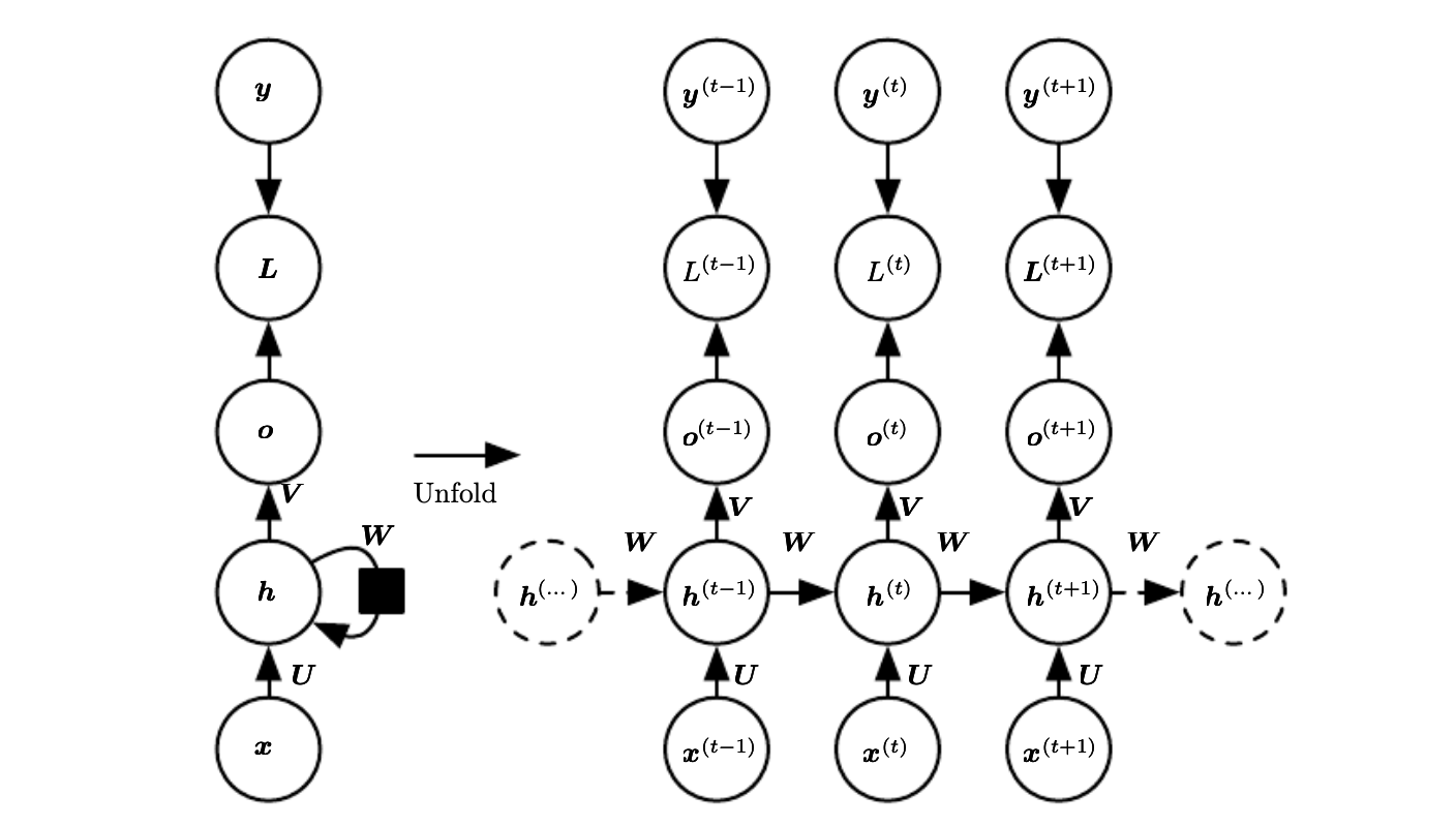
We can then apply the softmax function operation as a post-processing step to obtain a vectire $\hat{y}$ of normalized probabilities over the output.

a^{(t)} = b + Wh^{t-1} + Ux^{t} \\ h^{(t)} = \tanh(a^{(t)}) \\ o^{(t)} = c + Vh^{(t)} \\ \hat{y}^{(t)} = \text{softmax}(o^{(t)})

The total loss for a given sequence of $x$ values paired with a sequence of $y$ values would then be just the sum of losses over all the time steps.

L(t) = - \sum_t \log p_{model}(y^{(t)} \mid \{x^{(1)}, x^{(2)}, \dots x^{(t)}\})

$\text{BPTT}$ - Back Propagation Through Time:

One simply applies the generalized back propagation algorithm to the unrolled computational graph. The use of back propagation to the unrolled graph is called the back propagation through time.

Gradients obtained by back propgation may then be used with any general purpose gradient based techniques to train an $\text{RNN}$ .

Recurrent Networks as Directed Graphical Models:

In principle it is possible to use any loss with a recurrent neural network. We usually wish to interpret the output of the RNN as a probability distribution and we usually use the cross entropy associated with that distribution to define the loss.

When we use use a predicitve log-likelihood training cost, we train the RNN to estimate the conditional distribution of the next sequence element $y^{(t)}$ given the past inputs

\log{p}(y^{(t)} \mid x^{(1)}, x^{(2)}, \dots x^{(t)})

When we feed the actual values $y$ back into the network, the directed graphical model conatins edges from all $y^{(i)}$ values in the past to the current $y^{(t)}$ value.

We can consider the case where the RNN models only a sequence of scalar random variables $\mathbb{Y} = \{y^{(1)}, y^{(2)}, \dots y^{(\tau)}\}$ with no additional inputs $x$ .

We can then write

P(\mathbb{Y}) = P(y^{(1)}, y^{(2)}, \dots y^{(\tau)})

Where

L^{(t)} = -\log P(y^{(t)} = \texttt{y}^{(t)} \mid \{y^{(1)}, y^{(2)}, \dots y^{(t-1)}\})

To complete our view of an RNN as a graphical model, we must decribe how to draw samples from the model. We must also have some mechanism for determining the length of the sequence.

One can add a special symbol that correspinds to the end of a sequence. When this symbol is generated the sampling process stops.

Another option is to add an extra bernoulli output to the model that represents the decision to either continue generation or halt the generation.

another way to determine the sequence length $\tau$ is to add an extra output to the model that predicts the integer $\tau$ itself. The model can sample a value of $\tau$ and then sample $\tau$ steps worth of data.

Modelling sequences Conditioned on Contexts:

In, general, RNNs allow the extension of the graphical model to represent conditional distribution over $y$ given $x$ .

In case of $RNN$ this can be acheived in different ways.

interactions

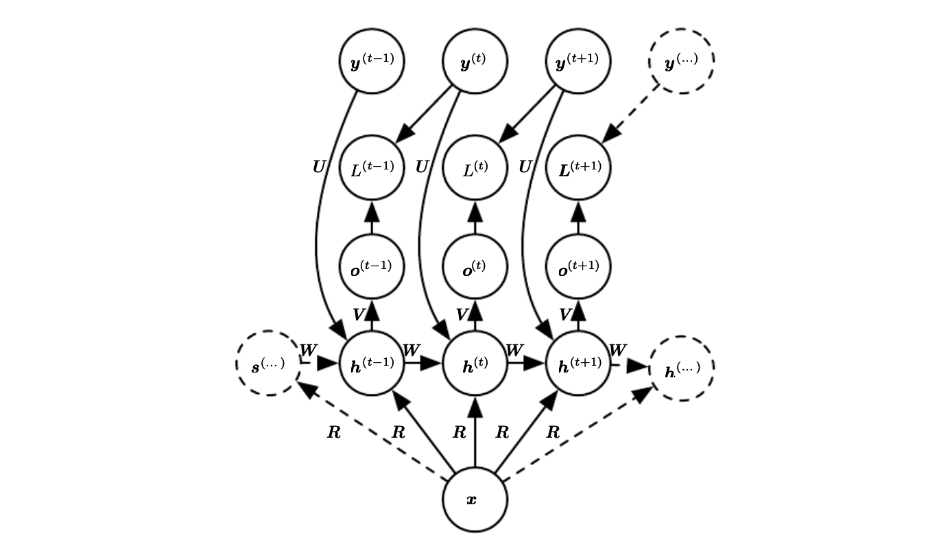
The interaction between the input $x$ and each hidden unit vector $h^{(t)}$ is parameterized by a newly introduced weight matrix $R$ . The product $x^{\top}R$ is added as additional input to the hidden units at every time step.

Rather than receiving only a single vector $x$ as input, RNN may receive a sequence of vectors $x^{(t)}$ as input. The model given above corresponds to a distribution that makes conditional independence assumptions.

conditional_independence

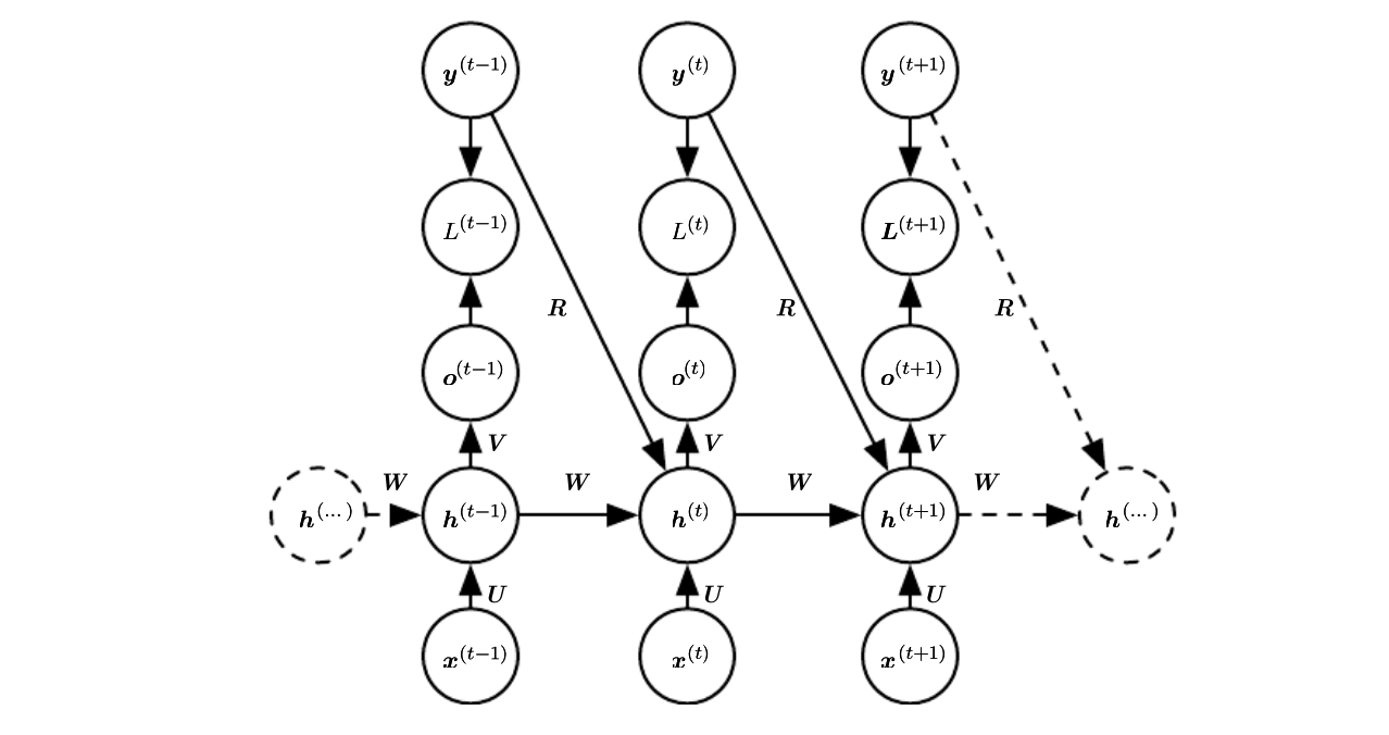
To remove conditional independence assumption, we can add connections from the output at time $t$ to a hidden unit at time $t+1$ .

Bidirectional RNNs:

bidirectional_rnn

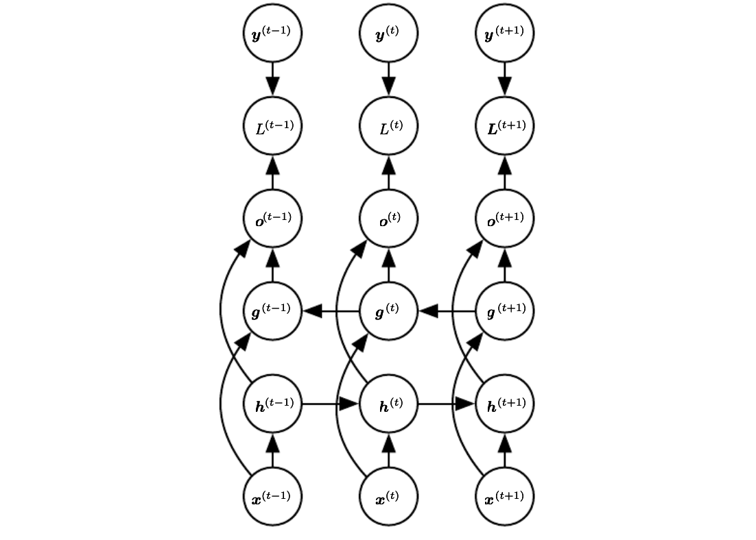
All of the RNNs considered up to now have a causal structure meaning that the state at time $t$ only captures information from the past and the present input.

However, in many applications we want to output a prediction whichi may depend on the whole input sequence.

Bidirectional RNNs were designed to address this need. They combine a RNN that moves forward with another RNN that moves backwards.

This allows the output unit to compute a representation that depends on both the past and the future but is most sensitive to the input values at time $t$ .

Encoder-Decoder Sequence-to-Sequence Architecture:

How an RNN can be trainied to map an input sequence to an output sequence which is not necessarily of the same length.

We introduct a context $C$ which is a vector or a sequence of vectors that summarize the input sequence.

The idea is very simple:

an encoder processes the input sequence and emits the context.
a decoder is conditioned on the context to generate the output sequence $Y$

If the context $C$ is a vector, then the decoder $RNN$ is simply a vector to sequence $RNN$ .

Thus input can be given in two ways:

As an initial state of the $RNN$
As an input to the hidden units at each time stamp.

One limitation is if the context $C$ has a dimension that is too small to properly summarize a long sequence.

Deep Recurrent Networks:

The computation in $RNN$ can be decomposed into three transformations:

Input to Hidden
Hidden to Hidden
Hidden to Output

Each of these block is associated with a single weight matrix. This is a transformation is represented by an affine transformation followed by a fixed non-linearity.

Would it be advantageous to introduce depth in each of these operations?

Recursive RNNs:

The Challenge of Long Term Dependencies:

The basic problem is that gradienst propagated over many stages tend to either vanish or explode.

the function composition employed by the $\text{RNN}$ resembles matrix multiplication

h^{(t)} = W^{\top} h^{(t-1)}

The recurrent relation applied $t$ times can be written as

h^{(t)} = (W^t)^{\top} h^{(0)} \\ h^{(t)} = Q^{\top} \Lambda^t Q h^{(0)}

How is this problem avoided in $\text{FFN}$ ?

Suppose that the weights $w^{(t)}$ are generated randomly,x independently from one another, with zero mean and variance $v$ . The variance of the product is $O(v^n)$ . To obtain some desired variance $v^*$ we may choose the individual weights with variance $v = \sqrt{v^*}$ . Thus very deep $\text{FFN}$ with carefully chosen scaling can this avoid the vanishing and exploding gradient problem.

Specifically, whenever the model is able to represent long term dependencies, the gradient of the long term interaction has exponentially smaller magnitude than the gradient of a short term interaction.

Thus it takes a very long time to learn the long-term dependencies.

the experimets show that as we increase the span of the dependencies that need to be captured, gradient based optimization becomes increasingly difficult.

Echo State Networks:

The recurrent weights mapping from $h^{(t-1)}$ to $h^{(t)}$ and the input weights mapping from $x^{(t)}$ to $h^{(t)}$ are the most difficult parameters to learn in a recurrent network.

ESN approach to avoiding this difficulty is to only learn the output weights ( $h(t)$ to $o(t)$ ). Set the recurrent weights such that the recurrent hidden units do a good job of capturing the history of the past inputs.

The training criterion may then be easlity designed to be convex as a function of the output weights.

The important question is how to set the input and recurrent weights so that a rich set of histories can be represented?

Leaky units and other strategies for Multiple Time Scales:

One way to deal with long-term dependencies is to design a model that operates at multiple time scales, so that some parts of the model operate at fine grained time scales, while other parts operate at coarse time scales and transfer information from the distant past to present.

1. Adding skip connections:

In ann ordinary $\text{RNN}$ a recurrent connection goes from a unit at time $t$ to a unit at time $t+1$ . It is possible to construct a recurrent networks with longer delays.

2. Leaky Units:

\mu^{(t)} = \alpha \mu^{(t-1)} + (1 - \alpha) x^{(t-1)}

When

$\alpha$ is near 1, remembers the information about the past
$\alpha$ is near 0, information about the past is discarded

Such a hidden unit is called a leaky unit.

Skip connections through time $d$ are a way of ensuring that a unit can always learn to be influence by the information from $d$ time steps earlier.

There are two basic strategies for setting the time constants. used by leaky units:

Manually fix them to values that remain constant.
Make time constants free parameters and learn time.

$\text{LSTM}$ and other gated $\text{RNN}s$ :

Leaky units allow the network to accumulate information. However, once that information is used, it might be useful to forget the old state.

Instead of manually deciding when to clear the state, we want the network to learn to decide when to do it. This is what gated $\text{RNN}s$ do

$\textbf{LSTM}$ :

A crucial addition has beem to make the weight of the connection from $h^{(t)}$ to $h^{(t+1)}$ be conditioned on the context $C$ .

By making the weights gated, the time scale of integraion can be changed dynamically.

Jaideep M. More

software engineer

Recurrent Neural Networks

Unfolding Computational Graphs:

Recurrent Neural Network:

$\text{BPTT}$ - Back Propagation Through Time:

Recurrent Networks as Directed Graphical Models:

Modelling sequences Conditioned on Contexts:

Bidirectional RNNs:

Encoder-Decoder Sequence-to-Sequence Architecture:

Deep Recurrent Networks:

Recursive RNNs:

The Challenge of Long Term Dependencies:

Echo State Networks:

Leaky units and other strategies for Multiple Time Scales:

1. Adding skip connections:

2. Leaky Units:

$\text{LSTM}$ and other gated $\text{RNN}s$ :

$\textbf{LSTM}$ :

Recurrent Neural Networks

Unfolding Computational Graphs:

Recurrent Neural Network:

BPTT\text{BPTT} - Back Propagation Through Time:

Recurrent Networks as Directed Graphical Models:

Modelling sequences Conditioned on Contexts:

Bidirectional RNNs:

Encoder-Decoder Sequence-to-Sequence Architecture:

Deep Recurrent Networks:

Recursive RNNs:

The Challenge of Long Term Dependencies:

Echo State Networks:

Leaky units and other strategies for Multiple Time Scales:

1. Adding skip connections:

2. Leaky Units:

LSTM\text{LSTM} and other gated RNNs\text{RNN}s:

LSTM\textbf{LSTM}:

$\text{BPTT}$ - Back Propagation Through Time:

$\text{LSTM}$ and other gated $\text{RNN}s$ :

$\textbf{LSTM}$ :