Machine Learning algorithms usually require a high amount of numerical computation. Common operations include optimization and solving systems of linear equations.

Evaluating mathematical functions on a digital computer can be difficult when function involves real numbers, which cannot be precisely represented.

This constitutes the rounding error. Rounding error is problematic, especially when it compounds across many operations and can cause algorithms that work in theory to fail in practice if they are not designed to minimize the rounding error.

Overflow and Underflow:

Underflow occurs when numbers near zero are rounded to zero. Many functions behave differently when their argument becomes zero. Ex: division by zero causes an error.

Overflow occurs when numbers with high magnitude are approximated as $\infty$ or $-\infty$. Further operation in these will lead to a Nan value.

One example of function that must be stabilised against underflow and overflow conditions is the softmax function.

When $\text{exp}$ are raised to the common power $c$ then:

1. when $c$ underflows and becomes $-\infty$ the denominator becomes $0$ and causes division by zero
2. when $c$ overflows and becomes $\infty$ then the whole expression becomes undefined.

Both of these issues are tackled by instead evaluating

The underflow issue is avoided as there is atleast one $\text{exp}$ raised to $0$ leading to $1$ in the denominator

The overflow issue is avoided as the highest power for $\text{exp}$ is $0$

We can simply rely on the low level libraries that provide stable implementations.

Poor Conditioning:

Conditioning refers to how rapidly a function changes with respect to small changes in its input.

Functions that change rapidly when their inputs are changed slightly can be problematic for scientific computation because rounding errors in the inputs can result in large changes in the output.

Gradient Based Optimization:

Optimization refers to the task of either minimizing or maximizing some function $f(x)$ by altering $x$

The function we want to minimize or maximize is called the objective function or criterion. When we are minimizing it, we may also call it the cost function, loss function or error function.

Suppose we have a function $y = f(x)$. the derivative $f'(x)$ gives the slope of $f(x)$ at point $x$. In other words, it specifies how to scale a small change in the input in order to obtain the corresponding change in the output: $f(x + \epsilon) \approx f(x) + \epsilon f'(x)$

The derivative is therefore useful for minimizing a function because it tells us how to change $x$ in order to make a small improvement in $y$. This technique is called gradient descent.

In the context of deep learning, we optimize functions that may have many local minima that are not optimal. This makes optimization difficult, especially when the input for a function is multi-dimensional. We therefore usually settle for finding a value of $f$ that is very low, but not necessarily minimal.

For functions with multiple inputs, we must make use of the concept of parital derivatives.

The gradient generalizes the notion of derivative to the case where the derivative is with respect to a vector: the gradient of $f$ is the vector containing all of the partial derivatives, denoted $\nabla_{x}f(x)$. Element $i$ of the gradient is the partial derivative of $f$ with respect to $x_{i}$.

In multiple dimensions, critical point is the point where all elements of the gradient are equal to zero.

the directional derivative in the direction $u$ (a unit vector) is the slope of the function $f$ in the direction $u$.

In other words the directional derivative is the derivative of $f(x + \alpha u)$, evaluated at $\alpha = 0$. Thus using the chain rule

To minimize $f$, we would like to find the direction in which $f$ decreases the fastest. We can do this using the directional derivative.

$\theta$ is the angle between the unit vector $u$ and the gradient

Substituting $\|u\|_{2} = 1$ and ignoring factors that do not depend on $u$, this simplifies to $\min_{u} \cos(\theta)$. This is minimized when $u$ points in direction opposite to the gradient.

The gradient always points to the uphill direction and thus we must always move in the negative gradient direction.

Thus to minimize the function $f$ we have to move in the direction opposite to the direction of the gradient

This is known as the method of steepest descent or gradient descent

$\epsilon$ is the learning rate, a positive scalar determining the size of the step.

Beyond the Gradient: Jacobian and Hessian Matrices

We are sometimes interested in a derivative of a derivative. This is known as second derivative.

The second derivative is important as it tells us whether a gradient step will cause as much of an improvement as we would expect based on the gradient alone.

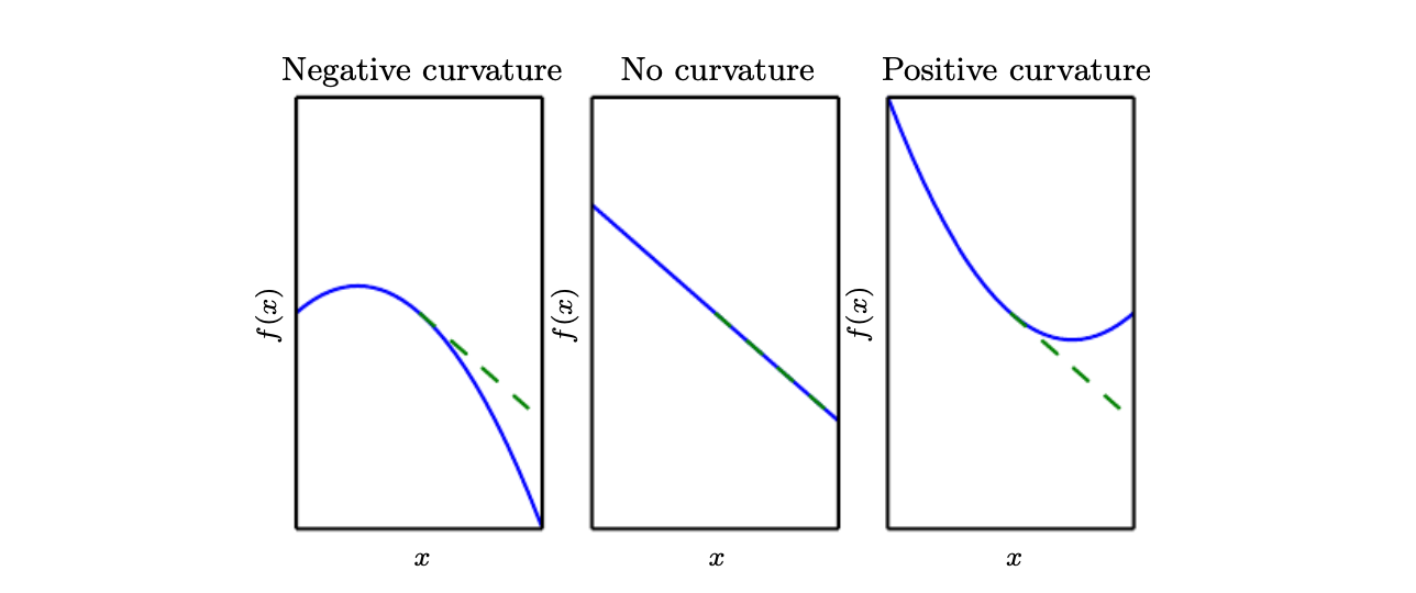
If a function has gradient equal to $1$ and if the second derivative

1. equal to $0$, then
   1. there is no curvature. It is a flat line.
   2. a step of $\epsilon$ in negative gradient decreases the value of the function by $\epsilon$
2. is negative, then
   1. the function curves downwards.
   2. the cost function will decrease by more than $\epsilon$
3. is positive, then
   1. the function curves upwards.
   2. the cost function will decrease by less than $\epsilon$

When our function has multiple inputs, there are many second derivatives. these derivatives can be collected together into a matrix called the Hessian Matrix.

When the second partial derivatives are continuous, the differential operations are commutative.

This implies that $H_{i, j} = H_{j, i}$ , so the Hessian matrix is symmetic.

Because the Hessian is real and symmetric we can decompose it into a set of real eigenvalues and an orthogonal basis of eigenvectors.

The second derivative in a specific direction represented by a unit vector $u$ is given by $u^{\top}Hu$.

• Case 1: $u$ is an eigen vector of $H$ then the second derivative is equal to the corresponding eigen value, $u_{i}^{\top}Hu_{i} = \lambda_{i}$

• Case 2: $u$ is not an eigen vector of $H$ then the second derivative is a weighted sum of the eigen values with weight being inversely proportional to the angle between $u$ and the corresponding eigen vector.

The directional second derivative can tell us how well we can expect a gradient step to perform. We can make use of Taylors Series to make an approximation of the function $f(x)$ around the current point $x^{(0)}$

Skipping the details $\dots$

The conclusion is that when the second derivative i.e. the Hessian is zero or negative, the learning rate and gradient will continue to minimize the function $f$

Now to apply the second derivative test to functions with multiple dimensions, we need to examine all of the second derivatives of the function.

We can generalize the second derivative test for multiple dimensions using the eigen decomposition of the Hessian.

When the gradient of the function is zero we can examine eigen values of the the Hessian

1. Hessian is positive definite: all the eigen values are positive. The point is local minimum
2. Hessian is negative definite: all the eigen values are negative. The point is local maximum
3. The test is inconclusive when there is atleast one zero eigenvalue and all of the non-zero eigen values have the same sign.

With multiple dimensions it becomes difficult to choose a good step size. The step size must be small enough to avoid overshooting the minimum.

This issue is resolved by using the information from the Hessian matrix to guide the search.

Newton’s method uses the second order taylors series to find the step size for minimizing the function.

It uses the Hessian as the step size at some point $x$.

So here the learning rate $\epsilon = H(f)(x)^{-1}$

Optimization function that uses only the gradient are called first-order optimization algorithms and algorithms such as Newtons method that also use the Hessian are called second-order optimization algorithms.