Introducution

The Task $T$:

Machine learning allows us to tackle tasks that are too difficult to solve with fixed program.

Machine learning tasks are described in terms of how the machine learning system should process an example.

An example is a collection of features that have been quanitatively measured from some object or event that we want the machine learning system to process.

The Performance Measure, $P$:

In order to evaluea the abilities of a machine learning algorithm, we must design a quantitative measure of its performance which is specific to the task $T$ being carried out.

Usually we are interested in how well the machine learning algorithm performs on data that it has not seen before, since this determines how well it will work when deployed in the real world.

The Experience $E$:

Machine learning algorithms can be broadly categorized as supervised or unsupervised based on whaat kind of experience they are allowed to have during the learning.

Unsupervised learning experience a dataset containing many features, then learn useful properties of the structure of this dataset.

Supervised learning experiece a dataset containing features, but each example is also associated with a label or target.

Linear Regression:

The goal is to build a system that can take a vector $x \in \mathbb{R}^n$ as input and predict the value of a scalar $y\in \mathbb{R}$.

In case of linear regression, the output is a linear function of the input.

We define the output to be

where $w \in \mathbb{R}^n$ is a vector of parameters

We can think of think of $w$ as a set of weights that determine how each feature affects the prediction.

We thus have a definition of our task $T$: to predict $y$ from $x$ by outputting $\hat{y} = w ^\top x$

Suppose we have a design matrix of $m$ examples that we will only use for evaluation how well the model performs. We also have a vector of regression targets $y$.

Because this dataset will only be used for evaluation, we call it the test set. We refer to the design matrix of inputs as $X^\text{(test)}$ and the vector of regression targets as $y^\text{(test)}$

One way of measuring the performance of the model is to compute the $\text{MSE}$ of the model on the test set.

So the error increases when the Euclidean distance between the predictions and the targets increase.

One intuitive way of minimizing the $\text{MSE}_{(test)}$ is to minimize the $\text{MSE}_{(train)}$.

To minimize $\text{MSE}_{(train)}$ we can simply solve for where its gradient is $0$:

we obtain,

Evaluating the above equation constitues a simple learning algorithm.

Capactiy, Overfitting and Underfitting:

Generalization: The ability to perform well on previously unobserved inputs is called generalization.

What seperates machine learning form optimization is that we want the generalizatiob error, also called the test error to be low as well.

We typically estimate the generalization error of a machine learning model by measuring its performance on the test set.

How can we affect the test set when we can only experience the training set?

The train set and the test set are generated by a probability distribution over datasets called the data generating process.

We make assumptions called the $i.i.d$ assumptions. Each example in the dataset is independent from each other and the training and test set are identically distributed.

The factors determining how well a machine learning algorithm will perform are its ability to:

1. Minimize the training error small
2. Minimze the gap between the training and test error

These two factors correspond to the two central challenges in machine learning underfitting and overfitting.

Underfitting:

Occurs when the model is not able to obtain a sufficiently low error on training set

Overfitting:

Occurs when the gap between the training and the test error if very large

We can control whether a model is more likely to underfit or overfit by altering its capacity. Informally, capacity is that ability of a model to fit a wide variety of functions.

Models with low capacity may fail to fit the training set and thus minimize the training error

Models with high capacoty can overfit my memorizing properties that do not serve them well for test set.

One way to control the capacity of a learning algorithm is by choosing its hypothesis space, the set of function that the learning algorithm is allowed to select.

Machine learning algorithm will perform well when the capacity is appropriately set according to the complexity of the task and the amount of the training set.

Capacity is not determined only by the choice of model. The model specifies the family of functions the learing algorithm can choose by varying the parameters. This is the representation capacity of the model.

In many cases, finding the best solution within this family is a very difficult optimization problem. These additional limitations, such as the imperfection of the optimization algorithm, mean that the effective capacity may be less than the representational capacity of the model family.

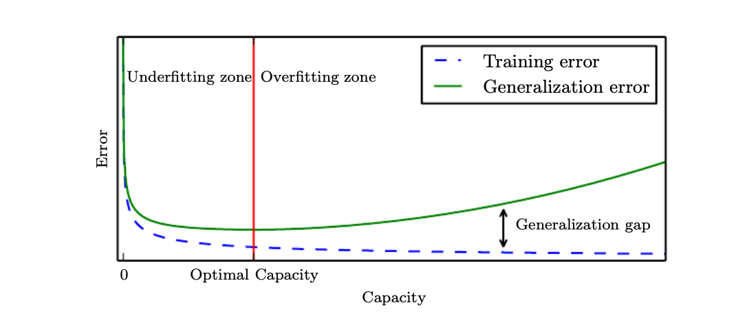
One important results in statistical learning theory shows that the gap between the training and the test error is upper bounded by a quantity that grows as the capacity increases and decreases as the training sample increases.

No Free Lunch Theorem:

States that, averaged over all possible data generating distributions, every classification algorithm has the same error rate when classifying previously unobserved points.

In other words no machine learning algorithm is universally any better than any other. The most sophisticated algorithm we can conceive has the same average performance as merely predicting that every point belongs to the same class.

Fortunately, these results hold only when we average over all possible datagenerating distributions. If we make assumptions on the distribution we encounter in the real-world appplications, we can design algorithm that perform well on these distributions.

Regularization:

Regularization is any modification we make to a learning algorithm that is intended to reduce the generalization error but not its training error.

The no free lunch theorem implies that we must design our machine learning algorithms to perform well on a specific task. We do so by specifying a set of preferences into the learning algorithm.

So far the only method of modifying a learning algorithm we have discussed is to increase or decrease the mdoels capacity by adding or removing the functions from its hypothesis space.

We can also give a learning algorithm a preference for one solution in its hypothesis space to another. This means that both functions are eligible but one is preferred.

Expressing preferences for one function over another is moregeneral way of controlling the models capacity than including or excluding members from the hypothesis space.

There are may ways of expressing preferneces, these difference approaches are known as regularization.

Hyperparameters and Validation Sets:

Most machien learning algorithms have severeal settings that we can use to control the behaviour of the learning algorithm. These settings are called hyperparameters.

The values of hyperparameters are not adapted by the learning algorithm.

More frequently, we do not learn the hyperparameter because it is not appropriate to learn the hyper parameter on the training set.

To solve this problem we need a validation set of examples that the training algorithm does not observe. The subset of data used to guide the selection of hyperparameters is called the validation set.

Earlier we discussed how a held-out test set, can be used to estimate the generalization error. It is imporatant that the test examples are not used in any way to make choices about the model, including its hyperparameters.

Cross Validation:

A small test set implies statistical uncertainty around the estimated average test error, making it difficult to claint that algorithm A performs better than algorithm B.

When the dataset is too small, there are alternative procedures which allow one to use all of the examples in the estimation of mean test error.

The most commpn of these is the k-fold cross validation procedure in which a data set is partitioned in to $k$ partitions. In iteration $i$ the $i$th partition is used as the test set and the remainder partitions are used for training.

Estimators, Bias and Variance:

Point Estimation:

Point estimation is the attempt to provide the single “best” prediction of some parameter or a vector of parameters.

Let $\{x^{(1)}, \dots x^{(m)}\}$ be set of $m$ independent and identically distributed ($i.i.d$) data points. A point estimator or statistic is any function of the data:

A good estimator is a function whose output is close to the true underlying $\theta$ that generated the training data.

In machine learning we are interested in approximating $f$ with a model or estimate $\hat f$. Function estimation is same as estimating a parameter $\theta$.

Linear regression is an example that may be interpreted as either estimating a parameter $w$ or estimating a function $\hat f$ mapping from $x$ to $y$.

Bias:

The bias of an estimator is defines as :

The expectation is over the data and $\theta$ is the true value of parameter used to define the data generating distribution.

An estimate $\hat \theta$ is said to be unbiased if $\text{bias}(\hat \theta) = 0$ i.e $\mathbb{E}(\hat{\theta}) = \theta$ and the estimator gives the best value of the parameter that approximates the function $f^*$. We want the estimator to exhibit low bias.

Variance and Standard Error:

The variance or the standard error of an estimator provides a measure of how we would expect the estimate we compute from data to vary as we independently resameple the dataset from the underlying data generating process.

The variance of an estimator is simply the variance where the random variable is the training set. Alternatively the square root of the variance is called the standard error.

Just as we want out estimator to exhibit low bias we would also like it have relatively low variance.

The expected degree of variation in the estimator is a source of error that we want to quantify.

Trading off bias and variance to minimize mean squared error:

Bias and Variance measure two different sources of error in an estimator. Bias measures the expexcted deviation from the true value of the function or parameter. Variance measures the deviation from the exptected estiamtor value that any particular sampling of the data is likely to cause.

The most common way to negotiate this tradeoff is to use cross validation. Alternatively, we can compare mean squared error MSE of the estimates:

Desirable estimators are those with small MSE and these are estimators that manage to keep both their bias and variance somewhat in check.

The relationship between bias and variance is tightly linked to the machine learning concepts of capacity, underfitting and overfitting.

In case where generalization error is measured by MSE, increaseing the capacity of the model tends to increase the variance and decrease bias.

Consistency:

Consistency ensures that the bias induced by the estimator is assured to diminish as the number of data examples grow.

the $\xrightarrow{p}$ means that the convergence is in probability i.e for any $\epsilon \gt 0$, $P(|\hat\theta_{m} - \theta| > \epsilon) \rightarrow 0$ as $m \rightarrow \infty$. This condition is called the consistency.

Maximum Likelihood Estimate:

How do we find a good estimate for a given model. The most common principle is the maximum likelihood principle.

Consider a set of $m$ examples $\mathbb{X} = \{x^{(1)}, \dots x^{(m)}\}$ drawn independently from the true but unknown data generating distribution $p_{data}(x)$

Let $p_{model}(x;\theta)$ be the parameteric family of probability distribution. $p_{model}(x; \theta)$ maps any $x$ to a real number that estimates the true probability $p_{data}(x)$

As logarithm is a monotone function we can take the logarithm of the likelihood and is does not change its $\arg \max$ but does transform the product into a sum.

One way to interpret maximum likelihood estimation is to view it as minimizing the dissimilarity between the empirical(or observed) distribution defined by the training set $\hat{p}_{data}$ and the model distribution $p_{model}$.

The left term is a function only of the data generating processs, not the model. Thus, while training the model we minimize the KL Divergence, thus we only need to minimize the negative log likelihood

Any loss consisting of negative log likelihood is a cross entropy between the empirical distribution defined by the training set and the model.

The maximum log likelihood can be readily generalized to the case where our goal is to estimate a conditional probability $P(y|x;\theta)$ inorder to predict $y$ given $x$

If $X$ represents all our inputs and $Y$ all our observed targets, then the conditional likelihood estimator is:

Under appropriate conditions, MLE has the property of consistency. These conditions are:

1. the true distribution $p_{data}$ must lie within the model family $p_{model}(.\theta).$
2. The true distribution $p_{data}$ must correspond to a single estimate (i.e. $\theta$).

Bayesian Statistics:

WE have discussed frequentist statistics and approach on estimating single values $\theta$, then making all predictions based on that one estimate

Another approach is to consider all possible values of $\theta$ when making a prediction. This is the domain of Bayesian Statistics.

The Bayesian uses probability to reflect the degrees of certainty of states of knowledge. On the other hand, the true parameter $\theta$ is unknown or uncertaing and thus is represented as a random variable.

Before observing the data, we represent our knowledge of $\theta$ using the prior probability distribution $p(\theta)$

Now consider that we have a set of data samples $\mathbb{X} = \{x^{(1)}, x^{(2)}, \dots, x^{(m)}\}$

Then we can recover the effect of the data on out belief about $\theta$ by combining the data likelihood $p(\mathbb{X} \mid \theta)$ with the prior $p(\theta)$ using the Bayes rule:

Relative to the maximum likelihood estimation, Bayesian estimation offers two important differences.

1. Unlike $\text{MLE}$, the Bayesian approach is to make predictions using a full distribution over $\theta$
2. The conrtibution of the prior distribution $p(\theta)$ the prior has an influence by shifting the mass density towards regions of the parameter space that are preferred.

Maximum A Posteriori $\text{MAP}$ Estimation:

While the most principle approach is to make predictions using the full Bayesian posteriori distribution over the parameter $\theta$, it is still often desirable to have single point estimation.

Rather than simply returning to the $\text{MLE}$, we can still gain some benefit of the Bayesian approach by allowing the prior to influence the choice of the point estimate.

One way to do is to choose the maximum a posteriori $\text{MAP }$point estimate. The $\text{MAP}$ chooses the point of maximal posterior probability.

$\text{MAP}$ Bayesian inference has the advantage of leveraging the information that is brought by the prior and cannot be found in the training data. This information helps to reduce the variance in the point estimate but causes increased bias.

Stochastic Gradient Descent:

Nearly all deep learning is powered by one very important algorithm: stochastic gradient descent $\text{SGD}$.

It is simply an extension of the Gradient descent algorithm.

A recurring problem in machine learning is that large training sets are necessary for good generalization, but large training sets are also more computationally expensive.

The insight of the $\text{SGD}$ is that the gradient is an expectation.

The expectation may be approximated using a small set of samples.

Specifically on each step of the algorithm, we can sample a minibath of examples $\mathbb{B} = \{x^{(1)}, x^{(1)}, \dots, x^{(m^\prime)}\}$ drawn uniformly from the training set.

The model can be trained on the entire training set but the updates are calculated only on the minibatch of examples.