Introduction:

Goal: the goal of a feedforward network is to approximate some function $f^{*}$

A feedforward network defines a mapping $y = f(x; \theta)$ and learns the values of the parameter $\theta$ that results in the best function approximation.

It is best to think of feedforward networks as function approximators that are designed to acheive statistical generalizaiton.

We begin with linear models and consider how to overcome their limitations. Linear models have the obvious defect that the model capacity is limited to linear functions, so the model cannot understand the interaction between any two input variables.

To extend the linear models to represent the non-linear functions of $x$, we can apply the linear model to a transformed input $\phi(x)$, where $\phi$ is a non-linear transformation.

The question is then how to choose the mapping $\phi$

1. We can use a very generic $\phi$ , such as the infinite dimensional. If $\phi(x)$ is of high enough dimension, we have enough capacity to fit the training set but the generalization to the test is poor.

2. We can manually engineer $\phi$. This approach requirs decades of human effort for each seperate task.

3. Strategy of deep learning is to learn $\phi$.

   In this approach we have the model $y = f(x;\theta, w) = \phi(x; \theta)^\top w$

   We now have parameter $\theta$ that we use to learn $\phi$ from a broad class of functions and $w$ that maps from $\phi(x)$ to $y$

   The $\phi$ defines a hidden layer. We parameterize the function as $\phi(x; \theta)$ and use an optimization algorithm to find $\theta$ that corresponds to a good representation.

This general principle of improving models by learning features extends beyond feedforward networks. It is a recurring theme of deep learning that applies to all of the kinds of models.

Learning XOR:

The XOR function provides the target function $y = f^{*}(x)$ that we want to learn. Our model provides a function $y = f(x; \theta)$ and our learning algorithm will adapt the parameters $\theta$ to make $f$ as similar as possible to our $f^{*}$

We can treat this problem as a regression problem. After fitting the regression model to this example the model simply outputs $0.5$ everywhere. This shows how a linear model is unable to represent a non-linear function.

We can solve this problem by applying the linear model to a transformed space in which it is able to represent the solution.

Specifically; we will introduce a very simple feedforward network with one hidden layer.

This network has a vector of hidden units $h$ that are computed by a function $f^{(1)}(x;W, c)$. The output layer is still a linear regression model, but now is applied to $h$ rather than $x$

The network now contains two functions:

1. $h = f^{(1)}(x;W, c)$ and
2. $y = f^{(2)}(h; w, b)$ in a chain.

What function should $f^{(1)}$ compute? If we use a linear function then the network as a whole computes only linear function of the input $x$

We must use a non-linear function that uses a affine transformation controlled by learned parameters, followed by a fixed non-linear activation function.

A gradient based approach can be used to find the parameters $(W, c)$ that produce best approximation for $f^{*}$

Gradient Based Learning:

The difference between the linear nodels and neural networks is that the nonlineraity of neural network causes loss functions to become non-convex.

A non-convex function is wavy - has some ‘valleys’ (local minima) that aren’t as deep as the overall deepest ‘valley’ (global minimum).

Stochastic Gradient Descent applied to non-convex loss function has no convergence guarantee, and is sensitive to the values of the initial parameters.

To apply gradient based learning for training neural network we must choose a cost function and coose how to represent the output of the model.

Cost Functions:

An important aspect of the design of deep neural network is the choice of the cost function.

In most cases our parametric model defines a distribution $p(y \mid x; \theta)$ and we simply use the maximum likelihood principle. This means we use the cross entropy between the training data and the models prediction as the cost function

The total cost function used to train a neural network will often combine one of the primary cost function described here with a regularization term.

Learning Conditional Distribution with $\text{MLE}$:

Most modern neural network are trained using maximum likelihood. Thus the cost functions is simply the negative log likelihood.

There exists equivalence between the $\text{MLE}$ with an output distribution and minimization of $\text{MSE}$ regardless of the $f(x;\theta)$.

An advantge of this approach of deriving the cost function for maximum likelihood is that it removes the burden of designing cost functions for each model.

Specifying a model $p(y \mid x)$ automatically determines a cost function $\log{p(y \mid x)}$

Output Units:

The choice of cost function is tightly coupled with the choice of output unit.

Most of the times for the cost function we use the cross entropy betwen the data distribution and the model distribution. The choice of how to represent the output then determines the form of the cross-entropy function.

We suppose that the feedforward network provides a set of hidden features defined by $h = f(x, \theta)$.

The role of the output layer is then to provide some additional transformation from the features to complete the task that the network must perform.

1. Linear Units for Gaussian Output Distribution:

One simple kind of output unit is an output unit based on an affine transformation with no non-linear activation function.

Linear output units are often used to produce the mean of a conditional Gaussian distribution.

$\text{MLE}$ is then equivalent to minimizing the $\text{MSE}$.

Because linear units do not saturate, they pose litle difficulty for gradient based optimization and may be used with a wide variety of optimization algorithms

2. Sigmoid units for Bernoulli Output Distribution:

Many tasks require predicting the value of a binary variable $y$.

A Bernoulli distribution is defined by just a single number. The neural net needs to only predict $P(y=1|x)$ and this value should be in the range $[0, 1]$.

We can think of the sigmoid output unit has having two components. First it uses a linear layer to compute

Next it uses a sigmoid activation function to normalize and convert $z$ into a probability.

We use a sigmoid output unit and combine it with $\text{MLE}$. Use of sigmoid function ensures that there is always a strong gradient to train the model effectively.

The loss function for bernoulli parameterized by signoid is

3. Softmax units for Multinoulli Output Distributions:

Softmax functions are most often used as the output of a classifier, to represent the probability distribution over $n$ different classes.

In case of binary variables, we wanted to produce a single number

To generalize to the case of a discrete variable with $n$ values, we now need to produce a vector $\hat y$ with

$\hat y_{i} = P(y=i \mid x)$. We require that not only the term $\hat y_{i}$ lies in the range $0$ to $1$ but also we want the sum of $\hat y_{i}$ to be equal to $1$.

First, a linear layer predicts the unnormalized log probabilities:

where $z_{i} = \log \tilde{P}(y=i \mid x)$. The softmax function can then exponentiate and normalize $z$ to obtain the desire $\hat y$.

For cost function

Hidden Units:

Now we turn to an issue that is unique to feedforward neural networks: how to choose the type of hidden unit to use in the hidden layers of the model.

It can be difficult to determine when to use which kind though rectified linear unit are usually an acceptable choice.

The design process consits of trial and errorm intuiting that a kind of hidden unit may work well, and then training a network with that kind of hidden unit and evaluatin its performance on a validation set.

Most hidden units can be described as accepting a vector of inputs $x$, computing an affine transformation $z = W^{\top}x + b$ and then applying an element-wise non-linear function $g(z)$.

Most hidden units are distinguished from one another only by the choice of the activation function $g(z)$

1. Rectified Linear Units:

Rectified Linear units are easy to optimize because they are similar to linear units.

ReLu are tupically used on top of a affine transformation:

When initializing the parameters of the affine transformation, it can be a good practive to set all elements of $b$ to a small positive value, such as $0.1$.

This makes it very likely that the ReLu will be active for most inputs and allow the derivatives to pass through.

One drawback of ReLu is that they cannot learn via gradient based methods on examples for which their activation is zero.

A variety of generalizations of ReLu guarantee that they receive gradient everywhere.

One such generalization is basd on using a non-zero slope $\alpha_i$ when $z_i < 0$.

1. Absolute Value Rectifications set $\alpha_i = -1$ obtains $g(z) = |z|$
2. Leaky ReLu sets $\alpha_i$ to a small positive value
3. parametric ReLu treats $\alpha_i$ as a learnable parameter

Maxout Units divide $z$ into groups of $k$ values. Each maxout unit then outputs the maximum element of one of these groups

Maxout units allow some statistical and computational advantages by requiring fewer parameters. Specifically, if the features captured by $n$ differenct linear filters can be summarized without losing information by taking the $\max$ over each group of $k$ features, then the next layer can get by with $k$ times fewer weights.

Rectified liner units and all of its generalizations are based on the principle that models are easier to optimize if their behavior is close to linear.

2. Logistic Sigmoid and Hyperbolic Tangent:

Prior to the introduction of rectified linear units, most neural networks used the logistic sigmoid activation function

or the hyperbolic tangent function

the widespread saturation of sigmoidal units can make gradient based learning very difficult. For this reason, their use as hidden units in feedforward networks is discouraged.

Their use as output units is compatible with gradient based learning using appropriate cost functions that can undo their saturation.

When a sigmoidal activation function must be used, the hyperbolic tangent activation function typically performs better than the logistic sigmoid

Some of the hidden units included in this list are not actually differentiable at all input points. In general, a function $g(z)$ has a left deriative defined by the slop of the function immediately at the left of $z$ and a right derivative defined by the slope of the function immediately to the right of $z$.

The functions used in the context of neural networks usually have defined left derivatives and defined right derivatives. Software implementations of neural network training usually return one of the one-sided derivatives rather than reporting that the derivative is undefined or raising an error.

this may be heuristically justified by observing that gradient based optimization is subjected to numerical error anyway. When a function is asked to evaluate $g(0)$, it is very ublikely that the underlying value was actually $0$. Instead, it could be a value $\epsilon$ rounded to $0$.

Architecture Design:

The word architecture refers to the overall structure of the network: how many units it should have and how these units should be connected.

Neural networks are organized into groups of units called layers. Most neural networks arrange these layers in a chain structure, with each layer being a function of the layer that precedes its.

In these chain based architectures, the main architectural considerations are to choose depth of the network and the width of each layer.

The ideal network architecture for a task must be found via experimentation guided by monitoring the validation set error.

Universal Approximation Properties and Depth:

The universal approximation theorem states that a feedforward network with a linear output layer and atleast one hidden layer with any “squashing” activation function can approximate any function, provided that the hidden layer has enough hidden units.

The universal approximation theorem means that regardless of what function we are trying to learn we know that a large enough network will be able to represent this function.

However, we are not guaranteed that the training algorithm will be able to learn that function. Learning can fail for two reasons:

1. The optimization algorithm used for training may not be able to find the value of parametes that correspond to the desired function.
2. The training algorithm may choose the wrong function due to overfitting.

The universal approximation theorem state that there exists a network to achieve any degree of accuracy but does not mention how large this network will be.

In summary, the network with a single hidden layer is sufficient to represent any function but the layer may be infeasibly large and may fail to learn and generalize correctly.

In many circumstances, using deeper models can reduce the number of units required to represent the desired function and can reduce the amount of generalization error.

We want to choose a deep model for statistical reasons. Any time we choose a specific machine learning algorithm, we are implicitly stating some set of prior beliefs we have about what kind of function the algorithm should learn. Choosing a deep model encodes a very general belief that the function we want to learn should involve composition of several simpler functions.

Other Architectural Considerations:

In general the layers need not be connected in a chain, even though this is the most common practice.

Many architectures build a main chain but then add extra architectural features to it, such as a skip connection going from layer $i$ to layer $i+2$ or higher.

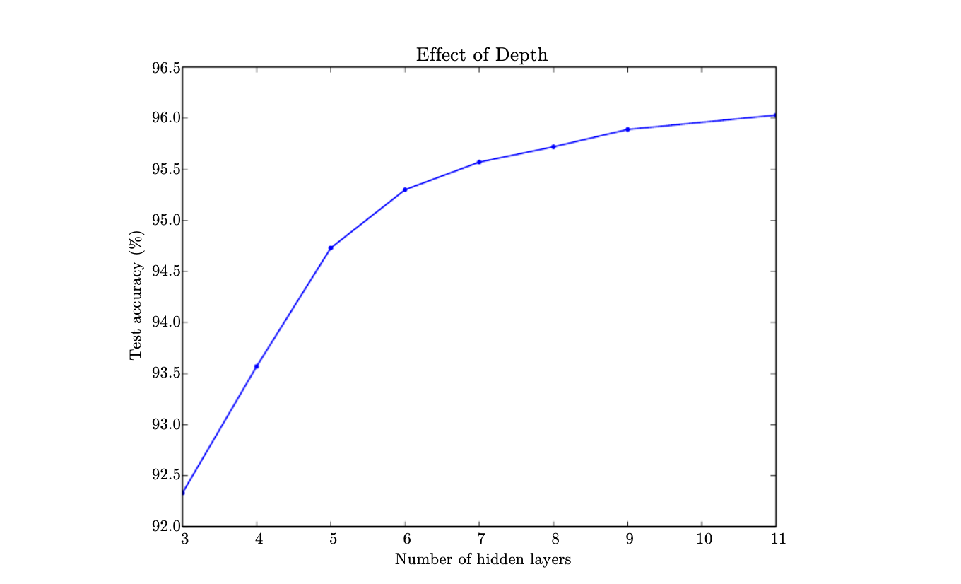
Test set accuracy increases with the increasing number of layers consistently. Deeper networks generalize better.

It expresses a belief that the function should consist of many simpler functions composed together. This could result either in learning a representation that is composed in turn of simpler representations.

However, increasing the number og parameters in layers without increasing the depth is not nearly as effective.

Back Propagation and Other Differentiation Algorithms:

The input $x$ provide the initial information that then propagats up to the hidden units at each layer and finally produces $\hat{y}$. This is forward propagation.

The back propagation allows the unformation from the cost to then flow backwards through the network, in order to compute the gradient.

Back propagatio refers only to the method of computing the gradient, while another algorithm, such as stochastic gradient descent is used to perform learning using this gradient.

In learning algorithm the gradient we most often require is the gradient of the cost function with respect to the parameters, $\nabla_{\theta}J(\theta)$

Chain rule of Calculus:

Back propagation is an algorithm that computes the chain rule, with a specific order of operations that is highly efficient.

Suppose:

1. $x \in \mathbb{R}^m, y \in \mathbb{R}^n, z \in \mathbb{R}$
2. $y = g(x)$
3. $z = f(y)$ then

such that

Thus, we can see that the gradient of a variable $x$ can be obtained by multiplying a Jacobian matrix $\frac{\partial y}{\partial x}$ by a gradient $\nabla_{y}z$.

The back propagation consists of performing such a Jacobian-gradient multiplication for each operation in the graph.

General Back Propagation:

To compute the gradient of some scalar $z$ with respect to one of its ancestors $x$ in the graph, we begin by observing $\frac{dz}{dz} = 1$.

We can then compute the gradient with respect to each parent of $z$ in the graph by multiplying the current gradient by the Jacobian of the operation that produced $z$

We continue multiplying by Jacobians travelling backwards through the graph in this way until we reach $x$.

For any node that may be reached by going backwards from $z$ from two or more paths, we sum the gradients from different paths at that node.