The name “convolutional neural network” indicates that the network employs a mathematical operation called convolution. Convolution is a specialized kind of linear operation.

Convolutional networks are simply neural networks that use convolution in place of general matrix multiplication in at least on of their layers.

The Convolution Operation:

Suppose we have a sensor that provides a reading $x(t)$ for every time instant $t$.

Our sensor is noisy and to obtain a less noisy output we want to average together several measurements. We want to have a weighted average. As the recent measurement is more accurate we want to give it more weight.

Thus, we can define a function that provides a smoothed sensor reading.

$w(t)$ provides the weight for the reading at time instant $t$

This operation is called convolution. The convolution operation is typically denoted with an asterisk.

In covolution network terminology, the first argument $x$ to the convolution is referred to as the input and the second argument $w$ is referred as the kernel. The output is sometimes referred to as the feature map.

Usually when we work with data, time will be discretized and our sensor will provide reading at regular intervals. The time index $t$ can then take only integer values. If we assume that $x$ and $w$ are defined only on integer $t$, we can define discrete convolution as:

In machine learning applications because each element of the input and kernel must be explicitly stored seperately, we assume that these functions are zero everywhere but the finite set of points for which we have the sensors reading.

This means that in prpactice we can implement the infinite summation as a summation over a finite number of array elements.

Finally, we use convolutions over more than one axis at a time.

Many neural network libraries implement a related function called the cross-correlation.

In the context of machine learning algorithm, the kernel is an multidimensional array with parameters that are adapted by the learning algorithm.

Discrete convolution can be viewed as multiplication by a matrix with the values of the matrix constrained to be equal to other entries.

For univariate discrete convolution, each row of the matrix is constrained to be equal to the row above shifted by one element. This is known as the Toeplitz Matrix.

Motivation:

Convolution leverages three important ideas that can help improve a machine learning system:

Sparse Interactions:

Traditional neural network layers use matrix multiplication by a matrix of parameters. Every output unit interacts with every input unit.

Convolutional networks, however have sparse interactions. This is obtianed by making the kernel smaller than the input.

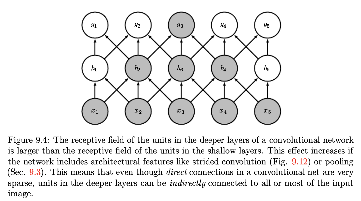
In a deep convolutional network, units in the deeper layers may indirectly interact with a larger portion of the input. This allows the network to efficiently describe complicated interactions between many variables by constructing such interactions from simple building blocks.

Parameter Sharing:

Parameter sharing refers to using the same parameter for more than one function in a model.

In a traditional neural net, each element of the weight matrix is used exactly once when computing the output of a layer.

In a conconvolutional neural net, each member of the kernel is used at every position of the input. The parameter sharing used by the convolution operation means that rather than learning a seperate set of parameters for every location, we learn only one set.

Equivariant Representations:

In case of convolution, the particular form of parameter sharing causes the layer to have a property called equivariance to translation.

To say a function is equivariant means that if the input changes, the output changes in the same way. Specifically, a function $f(x)$ is equivariant to a function $g(x)$ if $f(g(x)) = g(f(x))$

If we apply a trasformation to out input $I$, then apply convolution, the result will be same as if we applied convolution to $I$ and then applied the transformation.

Convolution is not naturally equivariant to some other transformations, such as changes in scale or rotation of an image. Other machanisms are necessary for handling these kinds of transformations.

Pooling:

A typical layer of convolutional network consists of three stages.

1. the layer performs several convolutions in parallel to produce a set of linear activations.
2. each linear activation is run through a nonlinear activation function. this stage is sometimes called the detector stage.
3. We use a pooling function to modify the output of the layer further.

A pooling function replaces the output of the net at a certain location with a summary statistic of the nearby outputs. Ex: the max pooling function reports the maximum output within a rectangular neighborhood.

In all cases, pooling helps to make the representation become approximately invariant to small translations of the input. Invariance to translation means that if we translate the input by small amount, the values of most of the pooled outputs do not change

Invariance to local translation can be very useful property if we care more about whether some feature is present than exactly where it is.

The use of pooling can be viewed as adding an infinitely strong prior that the function the layer learns must be invariant to small translations

Pooling over spatial regions produces invariance to translation, but if we pool over the output of seperately parameterized convolutions, the features can learn which transformation to become invariant to.

For many tasks, pooling is an essential for handling inputs of varying size. If we want to classify images of variable size, the input to the classification layer must have a fixed size.

This is usually accomplished by varying the size of an offset between pooling regions so that the classification layer always receive the same number of summary statistics.

Ex: The final pooling layer may be defined to output four sets of summary statistics, one for each quadrant of an image, regardless the size of the image.

Convolution and Pooling as an infinitely strong prior:

Prior probability distribution is a probability distribution over the parameters of a model that encodes our beliefs about what models are reasonable, before we have seen the data.

Priors can be considered strong or weak depending on how concentrated the probability density in the prior is. A strong prior has a very low entropy and such a prior plays an active role in determining where the parameters end up.

An infinitely strong prior places zero probability on some parameters and says that these parameters are completely forbiddenm regardless of how much support they get from the data.

We can think of convolution as introducing an infinitely strong prior. This prior says that the function the layer should learn contains only local interactions and is equivalent to translation. Likewise, the use of pooling is an infinitely strong prior that each unit should be invariant to small translations.

Thinking of the CNN as a fully connected net with infinitely strong prior can offer some key insights. one key insight is, if a task relies on preserving precise spatial information, then using pooling on all features can increase the training error

Variants of the Basic Convolution Function:

First when we refer to convolution in the context of neural networks, we usually mean an operation that consists of many applications of convolution in parallel. Usually we want each layer of our network to extract many kinds of features, at many locations.

In a multilayer convolutional network, the input to the second layer is the output of the first layer, which usually has the output of many different convolutions at each position.

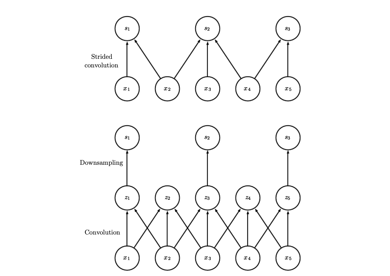
We may want to skip over some positions of the kernel in order to reduce the computational cost. We can think of this as downsampling the output of the fill convolution function.

If we want to sample only every $s$ pixels in each direction in the output, we can define a downsampled convolution function. We refer to $s$ as the stride of this downsampled convolution.

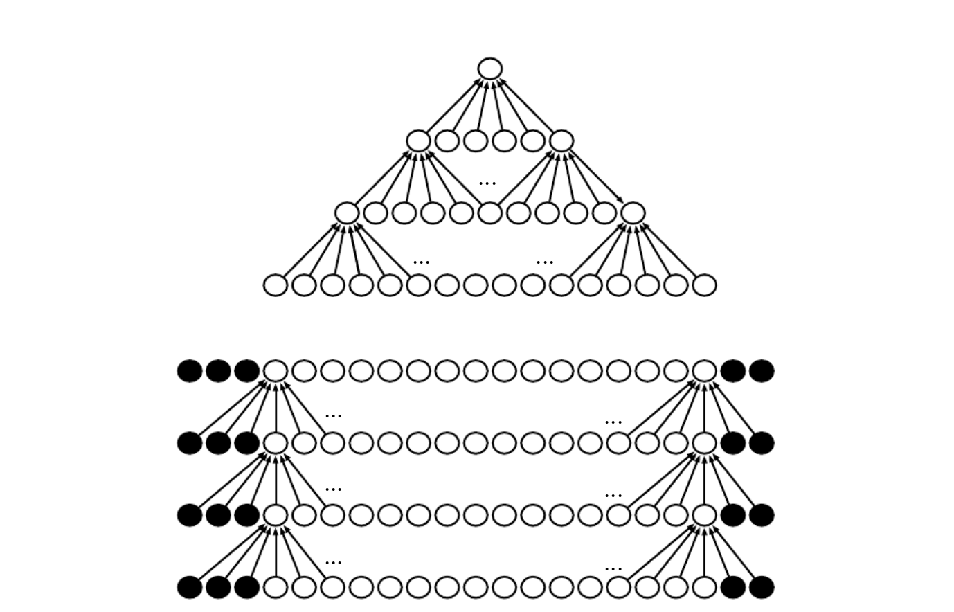
One essential feature of any convolutional network implementation is the ability to implicitly zero pad the input in order to make it wider. Without this feature the width of the representation shrinks.

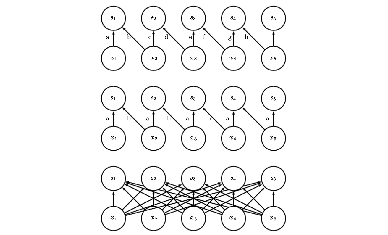
In some cases we do not actually want to use convolution but rather locally connected layers. This is sometimes also called unshared convolution, because it is a similar operation to discrete convolution with a small kernel but without sharing parameters across locations.

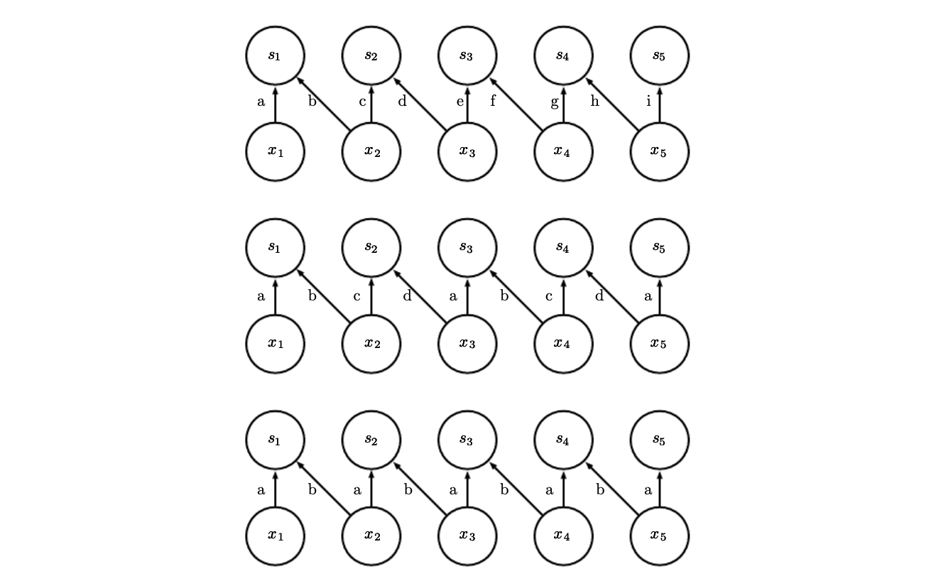
Tiled convolution offers a compromise between a convolutional layer and a locally connected layer. Rather than learning a seperate set of weights every spatial location, we learn a set of kernels that we rotate through as we move through space.

Structured Outputs:

Convolutional networks can be used to output a high dimensional, structured object, rahter than just predicting a class label for a classification task or a real value for a regression task.

Example we can emit a tensor $\mathbf{S}$, where $\mathbf{S}_{i, j, k}$ is the probability that pixel $(j, k)$ of the input to the network belongs to class $i$.

Efficient Convolution Algorithms:

Convolution is equivalent to

1. Converting both the input and kernel to frequency domain using Fourier transform
2. Perform pair wise multiplication of the two signals
3. Converting back to the time domain using inverse fourier transform.