1. Data Flow Analysis
   1. Dead Code Analysis
   2. Definite Assignment
2. Lattices and Fix point of monotone function
   1. Algorithms
3. Constant Propagation
   1. Unreachable Code
   2. Domain Cooperation (Unreachable code and Constant Propagation)
4. Abstract Interpretation
5. Pentagons and Bound Checking
6. Global Value Numbering

Dead Code Analysis:

Goal: To eliminate the computation whose result is unused

Definition: A variable $x$ is live at a program point in the CFG if there is a path from this program point to another program point where this variable is used which is not a definition.

Soundness: We must not eliminate computations whose result are live. Every over approximation is sound while eliminating dead code,

How do we find the set of live variables?

To determine the set of live variable at a program point $p$. For every variable $v$, we look at all the paths from point $p$ as the source. If we find any path where the variable is used $v_{1} \leftarrow v$ . Then the variable $v$ is live at that program point $p$.

A Local Approach:

For an edge $(u, v)$ in the CFG, assume we know the set of live variables at program point $v$. Then we can calculate the set of the live variables at $u$ using this information.

for every vertex $v$ that can be reached by $u$

The in-equation system:

Our in-equation system has an equation for each edge in the CFG.

For each node we $u$ can write the in-equation as the union of all the edges of the form $(u, v)$

We can use a function $\mathbb{L}$ that maps the set of program points $V$ to a set of variables that are live at that program point.

A trivial example of $\mathbb{L}$ maps each program point to the complete set of variables (all the variables are live at all the program points).

$\text{LV}$ is a transformer function. Takes in a particular mapping of program points to the set of live variables and transforms it into a new mapping.

NOTE: The best solution for the set of live variables $\mathbb{L}$ is obtained by the LFP of the $\text{LV}$

Definite Assignment:

Goal: Check that on each path to use a variable, the variable has been defined before the use.

Definition: A variable $x$ is definitely assigned at program point $p$ if every path from $r$ (root of the CFG) to $p$ contains a definition of $x$

Soundness: Every non-definitely assigned variable must be reported. warning about a definitely assigned variable is tolerable.

Thus, every under approximation of definitely assigned variables is sound.

A Local Approach:

For an edge $(u, v)$ in the CFG, assume we know the set of definitely assigned variables at program point $u$. Then we can calculate the set of the definitely assigned variables at $v$ using this information.

for every vertex $v$ that can be reached by $u$

The in-equation system:

Our in-equation system has an equation for each edge in the CFG.

For each node we $v$ can write the in-equation as the intersection of all the edges of the form $(u, v)$

We can use a function $\mathbb{A}$ that maps the set of program points $V$ to a set of variables that are live at that program point.

A trivial example of $\mathbb{A}$ maps each program point to the empty set of variables (all the variables are not assigned at all the program points).

$\text{DA}$ is a transformer function. Takes in a particular mapping of program points to the set of definitely assigned variables and transforms it into a new mapping.

Open Question:

So far we have the following:

1. Analysis Domain,(For Liveness $\mathbb{L}: V \rightarrow \mathscr{P}(\text{Vars})$): Gives the info derived about the program
2. Transfer function on the edges (For liveness $\text{lv}_{uv}$)
3. A join operator compatible with the order of the in-equation ($\bigcup$ for Liveness).
4. Using both we can build the single big function ($\text{LV}$)

How do we compute a solution for the in-equation systems?

Lattices and Fix-points of Monotone Functions:

• Lattice: A POSET(Set of elements $P$, ordering relation $\le$) is called a Lattice. Iff for every pair of element $\{x, y\}$ there exists a $\bigvee \{x, y\}$ and $\bigwedge \{x, y\}$

• Complete Lattice: A Lattice is called a complete lattice iff for every $S \subseteq P$ . $S$ is a Lattice.

• Conditions for Completeness: Let $(P, \le)$ be an ordered set, then the following statements are equivalent.

  1. $P$ is a complete lattice
  2. for every $S \subseteq P$ there exists a $\bigvee$ (By dual $\bigwedge$ exists).

• ACC - Ascending Chain Conditions: An ordered set $P$ fulfils the ascending chain condition, if for every sequence

  $$x_1 \le x_2 \cdots x_n \le x_i \in P$$

  then there exists $k \in \mathbb{N}$ such that $x_{k} = x_{k+1} = \cdots$

• Lifting: Let $(P, \le)$ be an ordered set/complete lattice. Let $V$ be a set. $(V\rightarrow P, \sqsubseteq)$ is an ordered set/complete lattice with

  $$a \sqsubseteq b : \ \ \forall v \in V, \ a(v) \le b(v)$$

• Knaster-Tarski Fixpoint Theorem: Let $L$ be a complete lattice and $f: L \rightarrow L$ be a monotone function. then

  $$\bigwedge \{ f(x) \le x \ |\ x \in L \}$$

  is the least fix point.

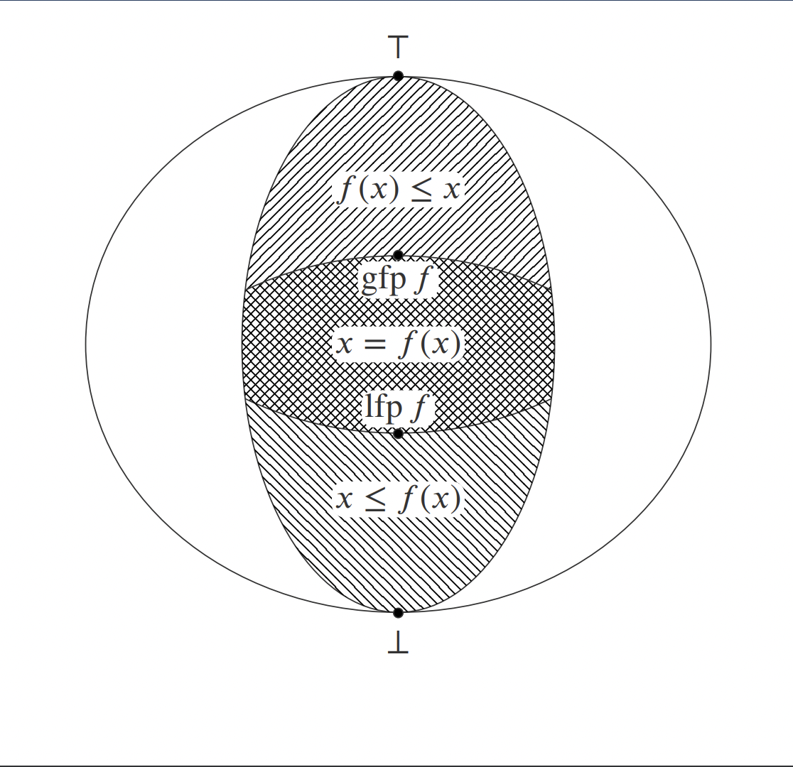
For the upper part of the diagram:

1. is the reductive part $f(x) \le x$
2. Is a sound solution for the Liveness analysis
3. $\text{lfp}$ is the best solution and contains the least number of variables live at each program point

For the lower part of the diagram:

1. is the expansive part $f(x) \ge x$
2. Is a sound solution for the Definite Assignment
3. $\text{gfp}$ is the best solution and contains the maximum number of variables defined at each program point.

Thus by Knaster-Tarski theorem we know about the existence of the best possible solution for the $LV$ and $DA$ analysis.

The question is how do we reach them.

Fixpoint by Iteration (Variation of Kleene’s theorem):

Let $L$ be a complete lattice that satisfies ACC and $f: L \rightarrow L$ a monotone function. then there exists a $k$ such that $f^k(\bot)$ is $\text{lfp}$ of $f$

The BIG Picture:

1. We require the analysis domain to be a complete lattice with ACC.

   for liveness and definite assignment, we had $V → \mathscr{P}(Vars)$ which is a complete lattice as $\mathscr{P}(vars)$ is a complete lattice with ACC.

2. We require every local edge transformer $f_{uv}$ to be a monotone function. Then the big Function $F$ ($\text{LV}$ and $\text{DA}$) are monotone.

3. WE compute the $F$’s fixpoint by using the Kleene’s theorem.

Chaotic Iteration:

$\text{lfp}\ F$ is the best most precise solution for our inequation system and thus the the most analysis.

We can reach this $\text{lfp}$ by. updating only one program point per step as long as we make progress

Constant Propagation:

Goal: Eliminate computations on the variables that are constant

Domain: $V \rightarrow (Vars \rightarrow Z_{\bot}^{\top})$ The domain of the analysis defines for each program point a information for each variable. The information either specifies a constant value or TOP(Not constant) or BOTTOM(not assigned)

Over approximates concrete states of program execution at program point.

$\top$ - there exists two states with different values for variable.

$\bot$ - the variable is not assigned for every state.

If there exists one state where the variable is assigned and is not assigned in all other states then, the un assigned state leads to undefined behaviour and are thus ignored. The analysis then considers the constant value and continues with the execution.

Functions on edges:

Abstract Expression Evaluation:

Here again we use the worklist algorithm to determine the constant values for the set of variables for the program points.

Unreachable Code:

Now we attempt to add another domain to the constant propagation and do unreachable code analysis in cooperation with the constant propagation analysis.

We use unreahability information to refine constantness and constantness to refine unreachability.

Additional domain:

Maps the set of program points to being either reachable ($\top_{U}$) or unreachable($\bot_{U}$).

Transfer Functions:

For every reachable program point $*u*$ we can determine the reachability information for $v$ as follows:

Domain Cooperation (Unreachable code and Constant Propagation):

When joining over all incoming abstract values in constant propagation we ignore predecessors that are unreachable.

NOTE: We cannot run this analysis one after the another as it wont lead to the optimal analysis. If there is no unreachability information then the constant propagation analysis will be poor which will lead to poor unreachability analysis.

Abstract Interpretation:

Some analysis domain are abstractions of concrete program properties.

Ex: For constant propagation $V \rightarrow (\text{Vars} \rightarrow \mathbb{Z}_{\bot}^{\top})$

A state ($\Sigma$) is a mapping $\text{Vars} \rightarrow \mathbb{Z}_{\bot}$ and exists in concrete program executions.

Ex: For constant propagation $\{x→\top, y→42, z→\bot\}$ represents all states where $\{\sigma | \sigma y=42 \land \sigma z=\bot \}$

We can use this information to prove program analysis correct with respect to the program semantics.

Concretisation(Constant Propagation):

Let $\mathbb{S} ⇒ (\mathscr{P}(\Sigma), \subseteq)$ be the complete lattice.

Let $\mathbb{C} = \{\text{Vars} \rightarrow Z_{\bot}^{\top}, \sqsubseteq\}$ be the constant propagation lattice.

WE define what an abstract element represents by defining a concretization function $\gamma_{\mathbb{S}}: \mathbb{C} \rightarrow \mathbb{S}$

$\gamma_{\mathbb{S}}(C\{x \mapsto 4\}) =$ Set of all states $\sigma$ where $Cx \mapsto 4$

$\gamma_{\mathbb{S}}$ is essentially taking in abstract information and giving us all the states in concrete program execution where the state is valid.

Correctness of edge transformers:

We can use the $\gamma$ to define the correctness criterion of the edge transformers.

Each control flow edge has a concrete edge transformer $f_{uv}:\Sigma \rightarrow \Sigma$

Each program analysis comes with a domain $\mathbb{A}$ and an abstract edge transformer $(f_{uv}^\#: \mathbb{A} → \mathbb{A})$ for each concrete effect $f_{uv}$

An abstract edge transformer $f_{uv}^{\#}$ is correct iff:

The above statement means that the states that are obtained by a concrete transformation under $f_{uv}$ are a subset of the states that can be obtained after abstract transformation under $f_{uv}^{\#}$

To prove the correctness for program analysis transformer we have to prove the above statement.

Finite Prefix Trace Semantics:

A configuration $\text{Conf} = V \times \Sigma$ is a pir of program point and a concrete state*.*

A trace $t$ is a sequence of configurations.

A finite prefix trace semantics is the set of all program executions.

We can define the following monotone function.

with

for an edge between program point $p$ with concrete state $\sigma$ and $q$ with concrete state $\sigma'$

Define the concretisation of constant propagation $V \rightarrow (Vars \rightarrow Z_{\bot}^{\top})$ to traces

The above statement means that if given some constant propagation information $C$ ($\text{Vars} \rightarrow Z_{\bot}^{\top}$) at a program point $p$ we can concretize it to a set of trace $\gamma(C)$ such that if $(p, \sigma) \in t$ then that state $\sigma$ appears in the set of concrete states that are obtained by that constant propagation information at that program point $p$; $\gamma_{\mathbb{S}}(C p)$.

Fixpoint Transfer:

Given a monotone function $\gamma:\mathbb{A} \rightarrow \mathbb{C}$ ($\mathbb{A}$ abstract, $\mathbb{C}$ concrete)

and two monotone functions $F:\mathbb{C} \rightarrow \mathbb{C}$ and $F^{\#}:\mathbb{A} \rightarrow \mathbb{A}$

for which the transformer correctness holds: $F \circ \gamma \subseteq \gamma \circ F^{\#}$

then,

Pentagons and Bound Checking:

For array accesses, a programming language like JAVA has to throw an exception if the array access is out of bounds.

So wherever there are array accesses a check is inserted to check the indexing.

There are some cases where the indexing is always in bound and the check is redundant.

With the interval analysis $(\text{Vars} \rightarrow (Z \times Z)_{\bot}^{\top})$, we only get the bound $[0, \infty]$.

This is not powerful enough to provide the relational information between the variables ($\texttt{i < arr.length}$)

Strict Upper Bounds Domain:

Represents strict inequalities, like $x \lt y$

Domain: $\text{Vars} \rightarrow \mathscr{P}(\text{Vars})$

Maps each variable $x$ to all the variables that are strictly greater than $x$

Concretisation: $\gamma_{\text{sub}} : s \mapsto \{\sigma | \forall x \ \ y : y \in s(x) \Rightarrow \sigma(x) < \sigma(y)\}$

Given an element $s$ from the analysis domain ($Vars \rightarrow P(vars)$) of SUB the concretisation function $\gamma_{sub}$ maps it to all the states $\sigma$ where the value of $y$ i.e. $\sigma(y)$ is strictly greater than the value of $x$ i.e. $\sigma(x)$

Join: $s \ \sqcup_{sub} \ t: \ \lambda x.(s(x) \cap t(x))$

$\top = \lambda x.\varnothing$ and $\bot = \lambda x.Vars$

the $\top$ denotes an absence of information about the values of the variables and hence assigns no ordering among the elements.

the $\bot$ is mapped to an empty state as there are no states where each variable is strictly greater than all other variables at the same time.

$\gamma_{sub}(\top): \sum$ i.e all the states and $\gamma_{sub}(\bot): \phi$

Closures: Because $\lt$ is transitive, there are many element in the SUB that concretise to the same set of states.

$s_{1} = [x \mapsto \{y\}, y \mapsto\{z\} ]$ and $s_{2} = [x \mapsto \{y, z\}, y \mapsto\{z\} ]$

for both of the above elements of analysis domain we get the same concretisation i.e. $\gamma_{sub}(s_{1}) = \gamma_{sub}(s_{2})$

Now, because $\gamma$ is a monotone function there exists a best abstraction $\alpha(c)$

Remember that $\alpha(c)$ is a function that maps the given set of concrete states to the best possible abstraction.

Therefore $(\alpha \circ \gamma)(s)$ gives the best abstraction for $\gamma (s)$ i.e. the best abstraction that represents the same concrete elements as $s$

$(\alpha \circ \gamma)$ is called the closure operator and is used to obtain the best abstraction for a given concretisation.

Why do I care to get the best abstraction when the concretisation leads to the same concrete states?

It actually makes difference when doing the join operation in the SUB domain.

To make join more precise once could compute the best abstractions using closure and then perform join.

However the closure operator is expensive and requires calculation of the closure of the relation represented by an abstract element

Reduced Product: Using SUB without intervals does not help in proving the array access in bounds. Information about constants is left-out. Hence we use both analysis domains at the same time: $\text{pentagons} = \text{SUB} \times \text{intervals}$

In the product, there are typically multiple abstract elements that are concretised to the same value:

Therefore, one also gets a closure operator that gives the best abstraction in $\text{SUB} \times \text{interval}$ domain

for a given abstraction

In Practice: Applying the closure operator is expensive.

To get the best precision, one has to do it before every operation: join and application of abstract transformer

In practice one uses a less precise but more efficient join. ex: ignore the SUB information for interval join.

Global Value Numbering:

Global Value Numbering $\Rightarrow$ Entire CFG

Local Value Numbering $\Rightarrow$ Inside a Basic Block

Local Value Numbering is aka CSE - Common Subexpression Elimination

Value Numbering:

Goal: Eliminate Redundant Computations

Find out if two variables have the same value at a given program point. (Undecidable).

Replace the later computations with the contents of the former.

We resort to Herbrand Equivalence:

We do not consider the interpretations of the operators.

Two expressions are equal if they are structurally equal.

Herbrand Interpretation:

Let $T$ be the set of terms over a set of variables.

The Herbrand interpretation $\mathscr{T}$ of an $n$-ary operator $\omega$ is given as

NOTE: The definition of a term is recursive. each term is composed of a set of terms.

Here the state $\sigma$ maps a variable to a term.

Herbrand Semantics $\langle t \rangle \sigma$ of a term t as follows

If the term $t$ is a variable then the value is equal to the value for that variable in the state $\sigma$

Else we recursively evaluate each term in the expression.

Two terms $t$ and $t^{'}$ are said to be Herbrand equivalent if for all states: $\langle t \rangle \sigma = \langle t^{'} \rangle \sigma$

Kildall’s Analysis:

Tracks Herbrand Equivalences with a forward analysis.

The equivalence relation is a congruence relation wrt operators in our expression language

For each operator $\omega$, each relation $R$ and for $e_{1}, e_{2}, ... \in \text{Vars} \cup T$

Abstract Transformer for an assignment $x \leftarrow t$

For the assignment operator $x \leftarrow t$ and a partition $R$, the new partition is calculated by relating all the terms $t_{1}$ and $t_{2}$ where replacing the term $x$ by $t$ does not change their equivalence.

Comments on Kildalls Analysis:

Kildalls analysis is sound and complete i.e it discovers all Herbrand equivalences in the program

Straight forward implementation exhibits explosion in the size of equivalence classes.

We can use a better data structure called SED (String Equivalence DAGs) to store the congruences but can still lead to exponential sized graphs.

The Alpern-Wegman-Zadeck Algorithm:

Generates incomplete and less precise value numbering analysis.

Flow insensitive: Does not compute the equivalences for every program point but sound for the whole program

Uses SSA (Static Single Assignment) which is a property of an Intermediate Representation.

In SSA each variable has a single program point where it is defined.

Interpret the SSA data dependence graph as FSM and minimize it.

In constrast to finite automata, we do not create two partitions but a class for every operator symbol.

Note that the $\phi$ is also treated as an operator.

Two $\phi$ from different blocks have to be in different classes

Optimistically place all nodes with the same operator symbol in the same class

Find the LFP

Successively split class when two nodes in the class are detected not equivalent